Module Detection
Compiled: 2022-08-02
Module_Detection.RmdHere we demonstrate gene program discovery using scale-free shared nearest neighbor network (SSN) analysis. The SSN method for gene program discovery was inspired by the established shared-nearest neighbor (SNN) framework used in single-cell analyses to reliably identify cell-to-cell distances in a sparse dataset, as well as the scale-free topology transformation used under the assumption that the frequency distribution of gene association in a transcriptomic network follows the power law.
In brief, the gene expression matrix is dimensionally reduced using principal component analysis (PCA). Each gene’s K-nearest neighbors (KNN) is then determined by Euclidean distance in PCA space. The resulting KNN graph is used to derive a shared nearest neighbor (SNN) graph by calculating the neighborhood overlap between each gene using the Jaccard similarity index. Adopting the framework from weighted gene correlation network analysis (WGCNA), an adjacency matrix that conforms to a scale-free topology is then constructed by raising the SNN graph to an optimized soft-thresholding power, which effectively accentuates the modularity of the network. The resulting adjacency matrix is used to construct the network UMAP embedding and to cluster genes into programs (or modules) by Louvain community detection. To reduce noise, genes with low connectivity (i.e., low network degree) are pruned so that only hub-like genes are retained for downstream annotation and analysis.
Load Seurat object
For this tutorial we will perform unsupervised module detection and annotation to characterize the biological processes that comprise the Human Gastrulation (Tyser 2021).
We start by reading in the data,
Feature Selection
We begin by identifying features used for downstream module detection. In general, lowly-expressed genes yield poorly constructed networks due to the high degree of sparsity. We offer 3 approaches to identifying genes for module detection:
-
Expression-based selection (“expr”): Feature
exceeding a minimal expression fraction (
min_pct) AND features that are highly-variable (FindVariableFeatures) are selected using this criterion. -
Highly-variable genes (“hvg”): Only features that
are highly-variable (
FindVariableFeatures) are selected using this criterion. -
Deviance-based selection: Features that are highly
deviant are selected using this criterion. Implemented with
scry::devianceFeatureSelection(..., fam = "binomial")
We can see that while there are some genes that overlap between the different approaches, there are many features that are also criterion-specific. In general, our expression-based selection criterion is the most widely encompassing approach, and is set as the default selection method.
# Expression-based feature selection
features_expr <- findNetworkFeatures(object = so.query, method = "expr", min_pct = 0.5)
# Highly-variable genes
features_hvg <- findNetworkFeatures(object = so.query, method = "hvg", n_features = 2000)
# Deviance-based feature selection
features_dev <- findNetworkFeatures(object = so.query, method = "deviance", n_features = 2000)
# examine overlap between feature sets
feature.list <- list(expr = features_expr, hvg = features_hvg, deviance = features_dev)
ggVennDiagram::ggVennDiagram(feature.list) + scale_color_manual(values = rep("white", 3))
Module Detection with SSN Workflow
We can now perform module detection using our scale-free
shared-nearest neighbor network (SSN) analysis pipeline, implemented in
the runSSN function.
so.gene <- runSSN(object = so.query, features = unique(c(features_hvg, features_dev)), scale_free = T,
robust_pca = F, data_type = "pearson", reprocess_sct = T, slot = c("scale"), batch_feature = NULL,
pca_var_explained = 0.9, optimize_resolution = T, target_purity = 0.8, step_size = 0.05, n_workers = parallel::detectCores(),
verbose = F)The resulting object contains a cell x feature Seurat
object, with the scale-free nearest neighbor graph stored in
so.gene@graphs[["RNA_snn_power"]] and the corresponding
UMAP embedding in so.gene@reductions[["umap"]].
We can visualize the scale-free optimization and transformation that was performed by calling the scale-free plots that are stored in the output object:
cowplot::plot_grid(so.gene@misc$scale_free$optimization.plot, so.gene@misc$scale_free$distribution.plot$`2`,
labels = "AUTO")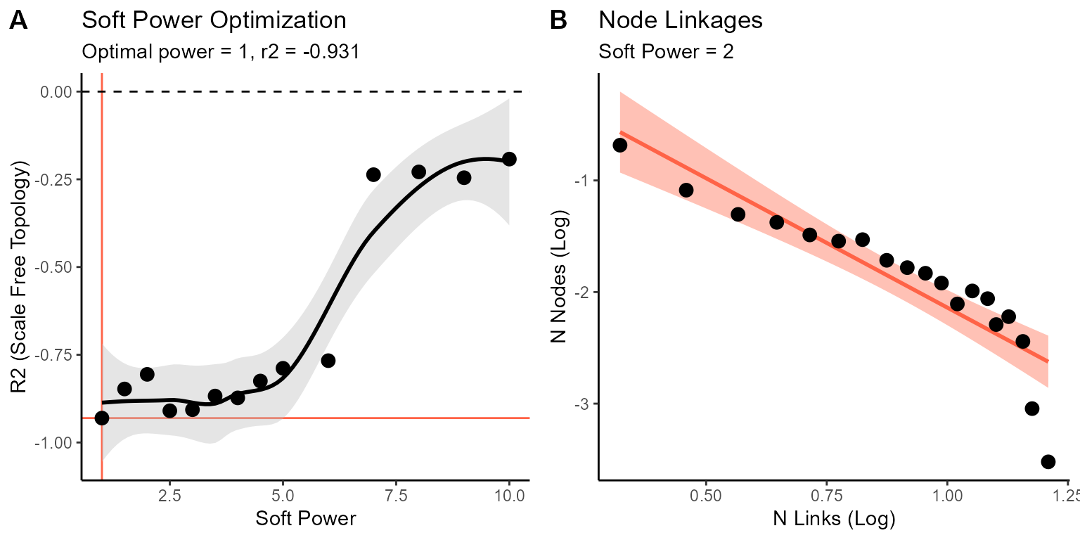
Using the UMAP layout and scale-free-transformed
shared-nearest-neighbor graph, we can visualize the network connectivity
using SSNConnectivity.
plt_connectivity <- SSNConnectivity(so.gene, quantile_threshold = 0.85, raster_dpi = 500)
plt_connectivity$plot_edge + labs(title = "Network Connectivity")
The module membership of each gene is stored in
so.gene@meta.data[["seurat_clusters"]] and can be
functionally-annotated as-is. However, we have introduced a filtering
step to clean up each module by pruning away features with low network
degree or connectivity. This is implemented using the
pruneSSN function.
# specify pruning threshold [0,1] (low values = less pruning, high values = more pruning)
prune.threshold <- 0.1
# get feature-specific connectivities (wi)
df.wi <- pruneSSN(object = so.gene, graph = "RNA_snn_power", prune.threshold = prune.threshold,
return.df = T)
# visualize
plt.prune <- df.wi %>%
ggplot(aes(x = wi_l2)) + geom_histogram(bins = 30) + geom_vline(xintercept = prune.threshold,
linetype = "dashed", color = "tomato") + labs(x = "Degree (L2 norm)", y = "Count", title = "Network Pruning",
subtitle = paste0(signif(100 * sum(df.wi$wi_l2 <= prune.threshold)/nrow(df.wi), 3), "% (", sum(df.wi$wi_l2 <=
prune.threshold), "/", nrow(df.wi), ") genes pruning")) + theme_miko(grid = T)
print(plt.prune)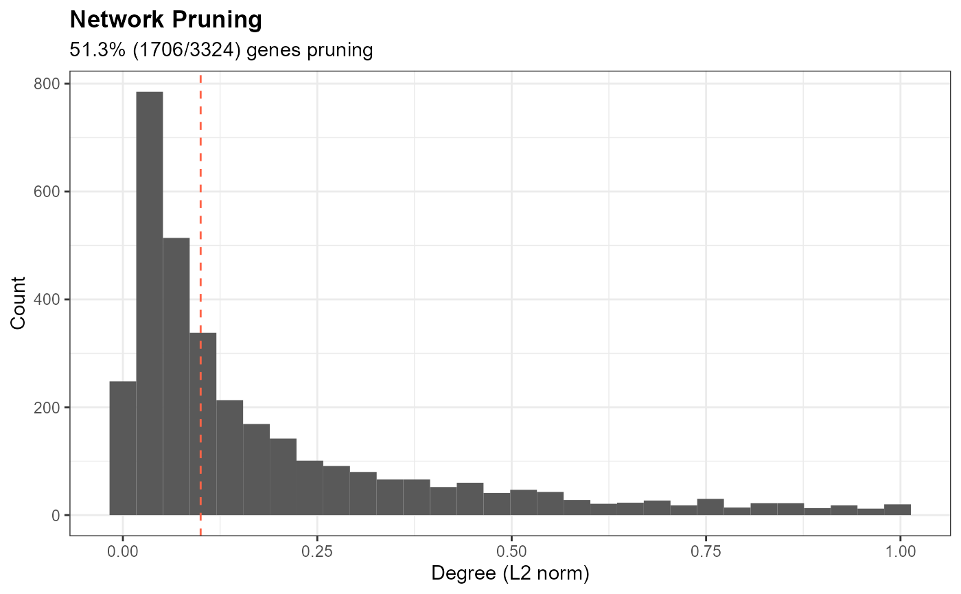
# get (pruned) gene module list
mod.list <- pruneSSN(object = so.gene, graph = "RNA_snn_power", prune.threshold = prune.threshold)
str(mod.list)## List of 11
## $ m0 : chr [1:424] "AARSD1" "AC009951.1" "AC010247.1" "AC018462.1" ...
## $ m1 : chr [1:307] "ABCA3" "AC002463.1" "AC002558.1" "AC004754.1" ...
## $ m2 : chr [1:232] "AAR2" "ABCF3" "AC007952.3" "AC093157.1" ...
## $ m3 : chr [1:166] "ABHD12" "AC006453.2" "ACMSD" "ACSL5" ...
## $ m4 : chr [1:70] "AC098934.1" "AL591806.3" "ARHGAP29" "ARL4C" ...
## $ m5 : chr [1:106] "ANLN" "ASF1B" "ASPM" "ATAD2" ...
## $ m6 : chr [1:76] "ABHD11" "AC007608.3" "AC008825.2" "AC022414.1" ...
## $ m7 : chr [1:79] "A2M" "ADORA3" "AGAP2.AS1" "AGR2" ...
## $ m8 : chr [1:56] "AC254813.2" "ADCY4" "AL158066.1" "ANGPTL4" ...
## $ m9 : chr [1:64] "AC090136.3" "AKAP14" "ANAPC5" "ANKRD66" ...
## $ m10: chr [1:38] "AC122719.1" "AGTR1" "AL513303.1" "ANXA8" ...An updated version of the connectivity plot can not be generated using the refined gene module sets.
plt_connectivity_with_features <- SSNConnectivity(so.gene, gene.list = mod.list, quantile_threshold = 0.85,
raster_dpi = 500, node.size.max = 6, node.size.min = 2, node.alpha = 0.6, node.weights = T,
node.color = "grey80")
# generate interactive network plot using plotly
plotly::ggplotly(plt_connectivity_with_features$plot_network)Finally, we summarize the expression and functional annotation of
each gene module using summarizeModules.
# summarize modules
ssn.summary <- summarizeModules(cell.object = so.query, gene.object = so.gene, gene.list = mod.list,
module.type = "ssn", n.workers = parallel::detectCores(), connectivity_plot = plt_connectivity_with_features$plot_edge)
# cluster-level heatmap of module activities
plt.ssn.gene.hm.expr <- heatmaply::heatmaply((ssn.summary$data.heatmap), scale = "column", scale_fill_gradient_fun = scale_fill_miko(),
xlab = "Module", ylab = "Cluster", main = "SSN Module Activity")
plt.ssn.gene.hm.expr
# get list of module-level summary plots
plt.ssn.gene <- ssn.summary$plt.summary
# assemble figure panels and visualize
x <- plt.ssn.gene$m10
cowplot::plot_grid(cowplot::plot_grid(NULL, x$cell.umap + theme(plot.title = element_text(hjust = 0.5)) +
theme(plot.subtitle = element_text(hjust = 0.5)), x$gene.umap + theme(plot.title = element_text(hjust = 0.5)) +
theme(plot.subtitle = element_text(hjust = 0.5)), NULL, nrow = 1, labels = c("", "A", "B", ""),
rel_widths = c(1, 4, 4, 1)), cowplot::plot_grid(x$bp.enrich, x$mf.enrich, x$cc.enrich, nrow = 1,
labels = c("C", "D", "E")), ncol = 1)