Cluster Optimization

Compiled: 2022-08-03

ScRNAseq-based cell type identification relies on unsupervised clustering methods; however, resulting cell clusters can vary drastically depending at what resolution is used to perform clustering. The specificity-based resolution selection criterion described here identifies cluster configurations coinciding with maximal marker specificity. Data is first clustered over a range of candidate resolutions, and the top specific marker in each cluster at each resolution is identified using the co-dependency index (CDI) DE method. Subsequently, specificity curves are generated and used to obtain resolution-specific specificity metrics. The resolution at which maximal specificity is observed is taken as the optimal resolution

For this tutorial we will analyze the Human Gastrulation dataset reported by Tyser 2021. The dataset consists of 1195 cells. We will identify the optimal clustering resolution using a specificity-based relution selection criterion.

We start by reading in the data and visualizing the annotated population.

# load package
library(scMiko)

# load human gastrulation data
so.query <- readRDS("../data/demo/so_tyser2021_220621.rds")

# visualize clusters
cluster.UMAP(so = so.query, group.by = "sub_cluster") + theme_void() + labs(title = "Tyser 2021",
    subtitle = "Human Gastrulation")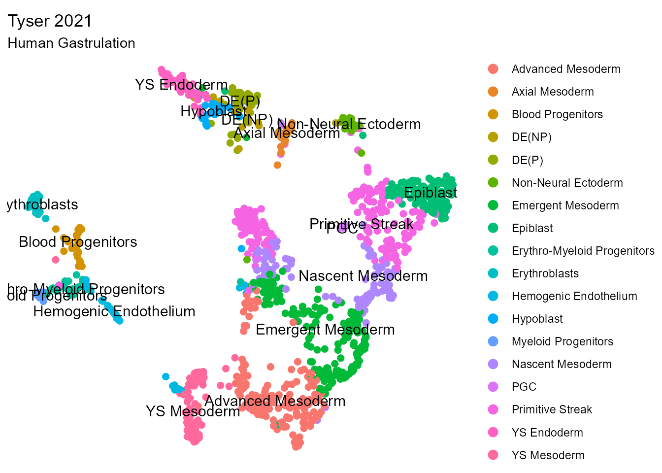

Multi-Resolution Clustering

Next, we cluster the data across a range of candidate resolutions. Cluster configurations can be visually assessed, and compared to cell populations annotated by the authors (above).

# clustering data
mc.list <- multiCluster(object = so.query, resolutions = c(0.05, 0.1, 0.2, 0.3, 0.4, 0.5, 0.75,
    1, 1.25, 1.5, 1.75, 2), assay = NULL, nworkers = 4, pca_var = 0.9, group_singletons = F, algorithm = 1,
    return_object = F)

# unwrap results
plt.umap_by_cluster <- mc.list$plots
so.query <- mc.list$object
cr_names <- mc.list$resolution_names
cluster.name <- mc.list$cluster_names
assay.pattern <- mc.list$assay_pattern

# visualize cluster configurations
cowplot::plot_grid(plotlist = lapply(plt.umap_by_cluster, function(x) {
    x + theme_void() + labs(title = NULL) + theme(legend.position = "none", plot.subtitle = element_text(hjust = 0.5))
}), ncol = 4)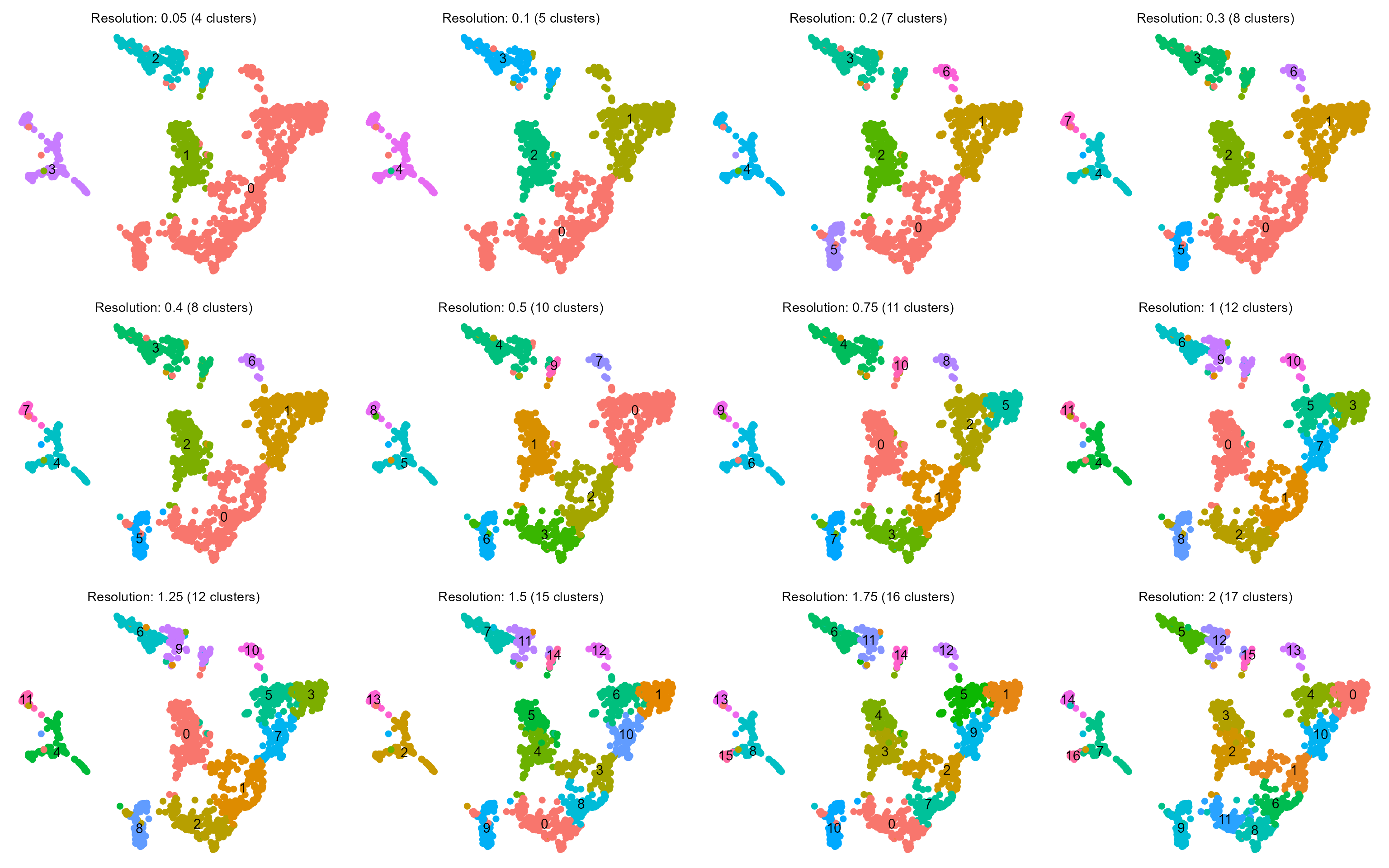

Specificity-Based Resolution Selection Criterion

Finally, for each cluster configuration, we compute a CDI-based specificity index. The optimal cluster resolution is determined based on the specificity profile. In this case we identify 0.5 as the optimal cluster resolution, yielding a specificity index of 0.614.

ms.list <- multiSpecificity(object = so.query, cluster_names = cluster.name, features = NULL, deg_prefilter = T,
    cdi_bins = seq(0, 1, by = 0.01), min.pct = 0.1, n.workers = 16, return_dotplot = T, verbose = T)

df.summary <- ms.list$specificity_summary
df.raw <- ms.list$specificity_raw
# plt.specificity.umap <- ms.list$umap_plot
plt.clust.spec <- ms.list$auc_plot
plt.auc.spec <- ms.list$resolution_plot
plt.auc.dot <- ms.list$dot_plot


max.auc = max(df.summary$auc)
speak <- df.summary$res[which.max(df.summary$auc)]


cowplot::plot_grid(plt.auc.spec + geom_hline(yintercept = max.auc, linetype = "dashed", color = "tomato") +
    geom_vline(xintercept = as.numeric(speak), linetype = "dashed", color = "tomato"), plt.clust.spec,
    plt.auc.dot$`0.5` + theme(legend.position = "right", axis.text.x = element_text(angle = 45,
        hjust = 1)), nrow = 1, rel_widths = c(1, 1.25, 1.25), labels = "AUTO")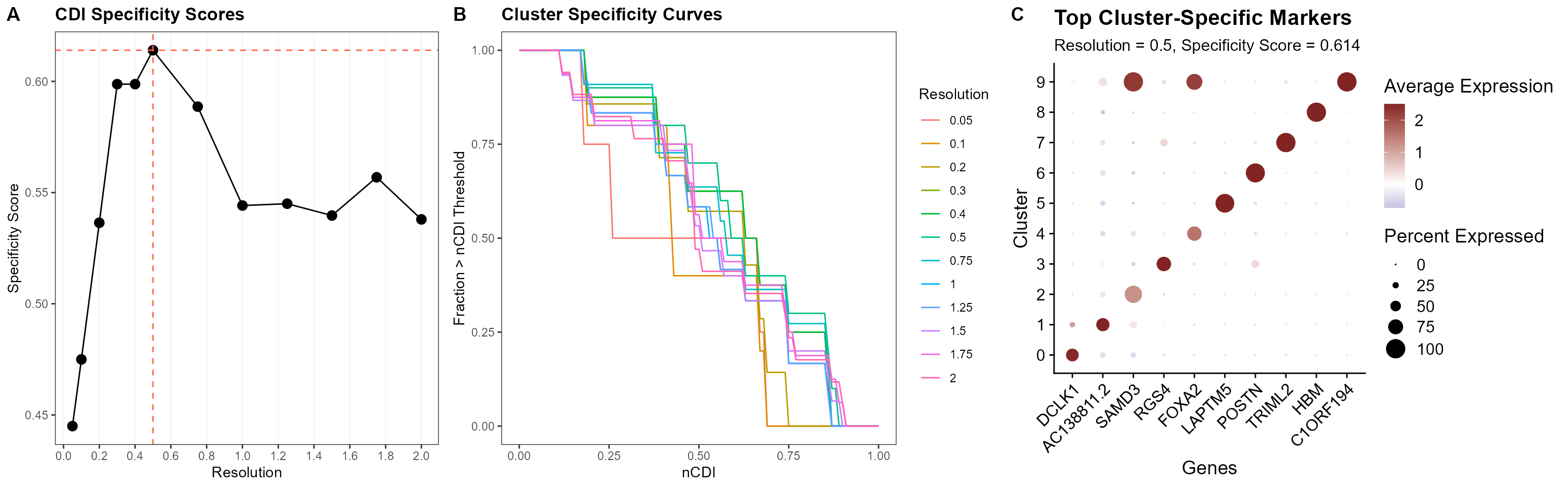

Multi-level resolutions

Acknowledging that there exist multiple levels of resolutions that are biologically relevant (e.g., cell types vs. cell subtypes), we can also specify valid cluster configurations at higher resolutions, as suggested by the “elbows” in the specificity plot. In the current dataset, we observe an “elbow” at a resolution of 1.0.

# plt.auc.dot$
cowplot::plot_grid(plt.auc.spec + geom_hline(yintercept = 0.544, linetype = "dashed", color = "tomato") +
    geom_vline(xintercept = 1, linetype = "dashed", color = "tomato"), plt.auc.dot$`1` + theme(legend.position = "right",
    axis.text.x = element_text(angle = 45, hjust = 1)), nrow = 1, rel_widths = c(1, 1.25, 1.25),
    labels = "AUTO")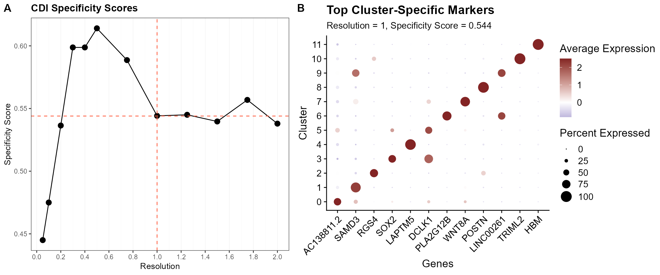

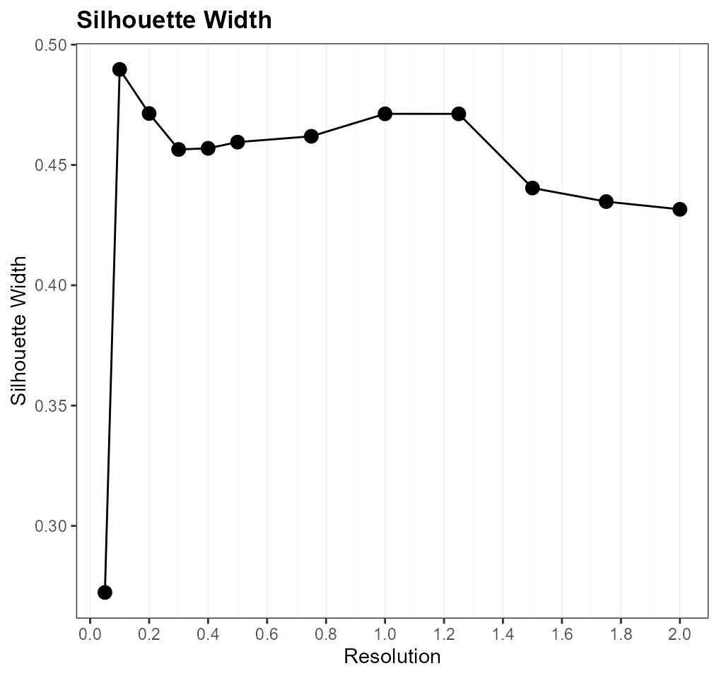
Alternative Method 1: Silhouette Width

For comparison, we also evaluate each cluster resolution using silhouette widths.

msil_list <- multiSilhouette(object = so.query, groups = cluster.name, assay_pattern = assay.pattern,
    verbose = T)

cowplot::plot_grid(plotlist = lapply(msil_list$silhouette_plots, function(x) {
    x + theme(plot.subtitle = element_text(hjust = 0.5))
}), ncol = 4)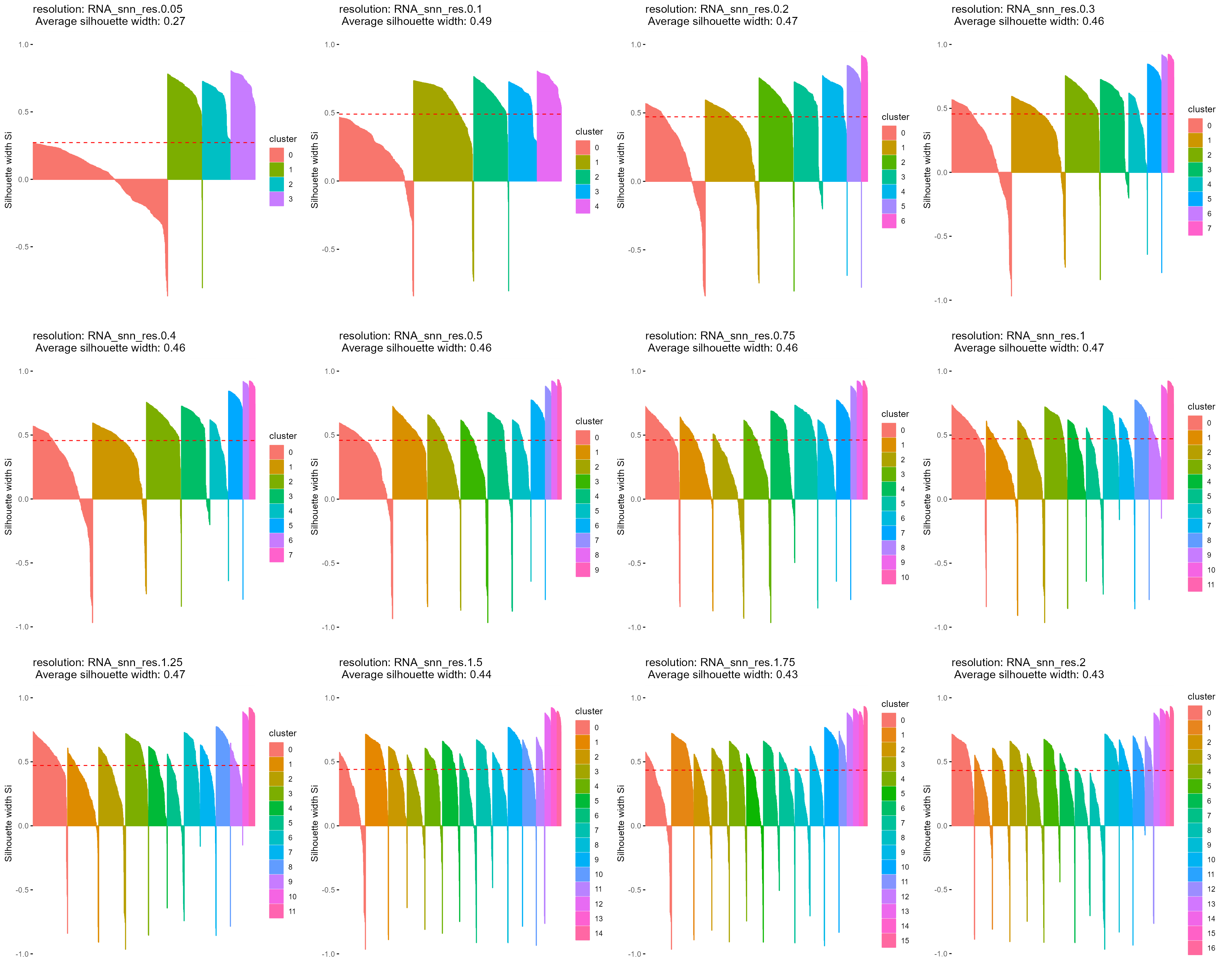

However, we can see that the silhouette width-based approach tends to favor lower resolutions that amalgamate cell clusters into larger populations.

msil_list$resolution_plot