Cell Annotation using the Miko Scoring Pipeline
Compiled: 2022-08-03
Cell_Annotation.RmdHere we demonstrate the Miko scoring pipeline, a cell cluster scoring method that accounts for variations in gene set sizes, while simultaneously offering a hypothesis-testing framework capable of rejecting non-significantly enriched gene sets. For a given single cell dataset, query and size-matched random gene sets are scored, and the difference between query and random module scores is scaled using the size-adjusted standard deviation estimate obtained from a gene set-size dependent null model to yield the Miko score. Scaling by the size-adjusted standard deviation estimate corrects for size-dependencies and results in a test statistic from which a p-value can be derived.
Using the Miko scoring pipeline, we will annotate the Human Gastrulation dataset reported by Tyser 2021. We start by reading in the data and visualizing the author-annotated population.
# load package
library(scMiko)

# load human gastrulation data
so.query <- readRDS("../data/demo/so_tyser2021_220621.rds")

# visualize annotated populations.
cluster.UMAP(so = so.query, group.by = "sub_cluster") + theme_void() + labs(title = "Tyser 2021",
    subtitle = "Human Gastrulation")
Prior to running the Miko scoring pipeline, you must ensure that the
loaded Seurat object has been clustered using
FindClusters() and that cluster information is available in
the ‘seurat_clusters’ meta data field.
# ensure that seurat_clusters are available
stopifnot("seurat_clusters" %in% colnames(so.query@meta.data))

# visualize seurat clusters
cluster.UMAP(so.query, group.by = "seurat_clusters")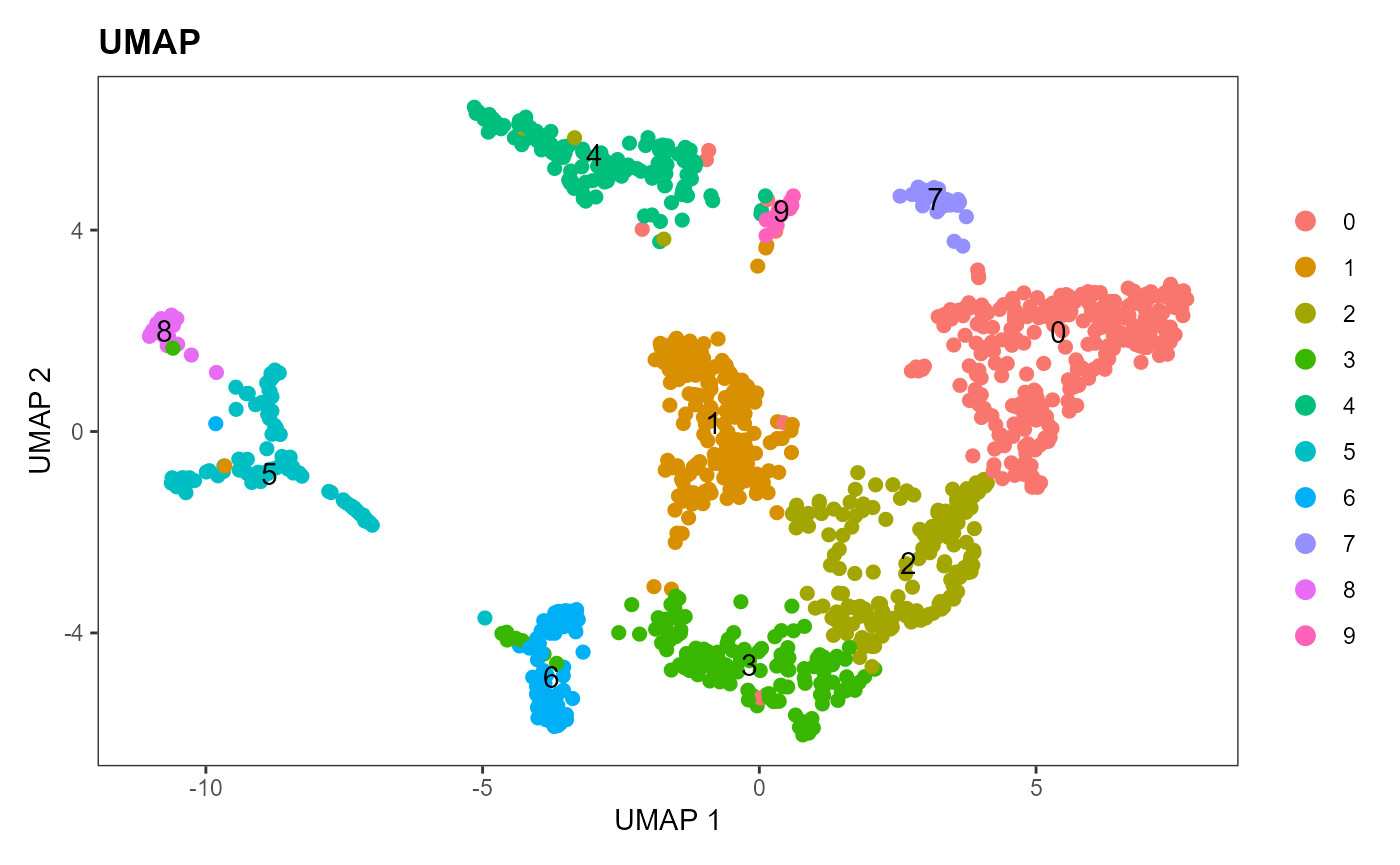
Prepare cell-type markers
Prior to performing marker-based cell-type annotation, we first prepare a comprehensive list of cell-type markers. We will use a cell-type catalog derived from multiple public scRNAseq atlases (see Cell-type marker catalog vignette for details).
In the absence of a-priori sample information, we would include all the cell-type markers in the catalog. However, given the known early embryonic age of the profiled sample, we will proceed with cell-markers derived from murine organogenesis (Cao 2019), human fetus (Cao 2020), developing murine brain (La Manno 2021), and murine gastrulation (Pijuan-Sala 2019):
# cell-type catalog
marker.df <- geneSets[["Cell_Catalog"]]
marker.list <- wideDF2namedList(marker.df)

# ensure that all genes are UPPER CASE (human)
marker.list <- lapply(marker.list, toupper)

# only include gene sets with more than 3 markers
marker.list <- marker.list[unlist(lapply(marker.list, length)) > 3]

# subset markers
marker.list <- marker.list[grepl("Cao2019|Cao2020|Manno|Pijuan", names(marker.list))]
Miko scoring pipeline
The miko scoring pipeline is a 3-step workflow that is implemented in
nullScore(), mikoScore(), and
sigScore() functions.
In step 1 we run nullScore(), which
fits a null model that corrects for gene set-size biases.
# step 1
ns.res <- nullScore(object = so.query, assay = DefaultAssay(so.query), n.replicate = 10, nbin = 24,
    min.gs.size = 2, max.gs.size = 200, step.size = 10, nworkers = 16, verbose = T, subsample.n = 5000)
From this example, the variance-gene set-size relationship can be appreciated in panel A and B. Panel C illustrates the correction that is applied to ensure that the null score variance is constant across all gene set sizes.
variance.mean.plot <- ns.res$variance.mean.plot
plt.null.model <- ns.res$mean.plot
plt.corrected.plot <- ns.res$corrected.plot

cowplot::plot_grid(variance.mean.plot + labs(subtitle = ""), plt.null.model, plt.corrected.plot +
    labs(title = "Gene Set-Size Corrected Null Scores", subtitle = ""), nrow = 1, align = "h", labels = "AUTO")
In step 2, cell-type marker sets are scored using
mikoScore().
# step 2
so.query_scored <- mikoScore(object = so.query, geneset = marker.list, nbin = 24, nullscore = ns.res,
    assay = DefaultAssay(so.query), nworkers = 18)
Finally, in step 3, we identify which cell-type
marker sets are significantly enriched in each cluster using
sigScore().
# step 3
score.result <- sigScore(object = so.query_scored, geneset = marker.list, reduction = "umap")

# visualize score.result$score_plot
Post-scoring filters
We use two additional post-scoring filters to fine tune which gene sets are enriched. The first is a coherence filter in which a positive correlation between component gene expression and the Miko score is enforced for a minimum fraction of component genes. The second is a frequent flier filter, which flags gene sets that exceed a minimum significance rate and represent gene sets that enrich across most cell clusters.
Coherence filter
raw.mat <- so.query_scored@misc[["raw_score"]]
colnames(raw.mat) <- gsub("raw_", "", colnames(raw.mat))

df.cscore <- coherentFraction(object = so.query_scored, score.matrix = raw.mat, nworkers = 16, method = "pearson",
    genelist = marker.list, assay = DefaultAssay(so.query_scored), slot = "data", subsample.cluster.n = 500)

df.score <- score.result$cluster_stats
df.score$gs <- df.score$name
df.score$cluster <- df.score$cluster
df.merge <- merge(df.cscore, df.score, by = c("gs", "cluster"))

df.merge$sig <- df.merge$coherence_fraction >= 0.8 & df.merge$miko_score > 0 & df.merge$fdr < 0.05
plt.score.vs.coh <- df.merge %>%
    ggplot(aes(x = (miko_score), y = coherence_fraction, label = gs, fill = sig)) + geom_point(pch = 21,
    color = "white", size = 2) + theme_miko(legend = T) + geom_hline(yintercept = 0) + geom_vline(xintercept = 0) +
    scale_fill_manual(values = c(`TRUE` = "tomato", `FALSE` = "grey")) + labs(x = "Miko Score",
    y = "Coherence Fraction", fill = "Enriched & Coherent\n(FDR<0.05)", title = "Coherent Enrichments",
    subtitle = paste0(100 * signif(sum(df.merge$sig, na.rm = T)/nrow(df.merge), 3), "% Significance Rate"))


plt.score.vs.coh
df.score_summary <- data.frame(cluster = df.merge$cluster, cell.type = df.merge$gs, miko_score = signif(df.merge$miko_score,
    3), p = signif(df.merge$p, 3), fdr = signif(df.merge$fdr, 3), coherence_fraction = signif(df.merge$coherence_fraction,
    3))
Frequent flier filter
ugrp <- unique(df.score_summary$cluster)
df.score_summary.sig <- df.score_summary %>%
    dplyr::filter(fdr < 0.05)
df.tally.ff <- as.data.frame(table(df.score_summary.sig$cell.type))
df.tally.ff$Freq2 <- df.tally.ff$Freq/length(ugrp)

ff.thresh <- 0.75
which.ff <- as.character(df.tally.ff$Var1[df.tally.ff$Freq2 >= ff.thresh])
df.score_summary$frequent_flier = (df.score_summary$cell.type %in% which.ff)
We can visualize the frequent flier distribution to verify that an appropriate frequent flier threshold was used. In the current sample, we can see that there are a subset of marker sets that enrich indiscriminately in all clusters. In this case a threshold of 0.75 was appropriate (the threshold usually varies 0.6-0.8).
plt.ff <- df.tally.ff %>%
    ggplot(aes(x = Freq2)) + geom_histogram(binwidth = 0.1) + geom_vline(xintercept = ff.thresh,
    linetype = "dashed", color = "tomato") + labs(title = "Frequent Flier Distribution", subtitle = paste0(signif(100 *
    sum(df.tally.ff$Freq2 > ff.thresh)/nrow(df.tally.ff), 3), "% enriched genesets are frequent fliers (significant > ",
    100 * ff.thresh, "% of clusters)"), x = "Proportion of significant clusters", y = "Number of gene sets") +
    theme_miko()
plt.ff
Interpretting Annotations
Annotations are interpreted using the following statistics:
- miko_score: cell-type marker enrichment score.
- p and fdr: p- and adjusted p-values (fdr) for determining significance.
-
coherence_fraction: Fraction of genes that are
correlated to aggregate gene set expression.
- frequent_flier: Flag specifying whether annotation exceeds a given significance rate (i.e., is non-specific).
Example thresholds: miko_score > 0, fdr < 0.05, coherence_fraction > 0.8, frequent_flier = F
The annotationCloud() function can be used to facilitate
visualization and interpretation of annotations.
   plt.cloud <- annotationCloud(object = so.query_scored,
                                object.group = "seurat_clusters",
                                score = df.score_summary$miko_score,
                                score.group = df.score_summary$cluster,
                                score.cell.type = df.score_summary$cell.type,
                                score.p = df.score_summary$p,
                                score.fdr = df.score_summary$fdr,
                                score.coherence.fraction = df.score_summary$coherence_fraction,
                                score.frequent.flier = df.score_summary$frequent_flier, #
                                fdr.correction = T,
                                p.threshold = 0.05,
                                coherence.threshold = 0.9,
                                show.n.terms = 15,
                                verbose = T)
Example 1
This is an example of a clean annotation. Consistently across marker sets derived from independent studies, we find that the population is enriched for erythroid/erythrocyte/’erythroblast markers. Accordingly, the original authors had annotated this cluster as erythroblasts.
plt.cloud[[9]]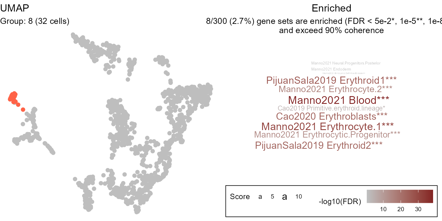
Example 2
In this example there is no consensus annotation. However we can see that annotations consistently identify mesenchymal-like annotations from multiple independent sources (e.g., Manno 2021 - mesenchymal progenitors; Cao 2019 - osteoblasts; Cao 2020 - smooth muscle cells; Pijuan-Sala - mesenchyme). Based on our annotations, we conclude that this cluster represents a mesenchymal population present during early human gastulation. The original authors had annotated this as Advanced Mesoderm.
plt.cloud[[4]]
Example 3
In this example the top annotations are Distal Visceral Endoderm and Embyonic Definitive Endoderm suggesting an endodermal identity. However we must be cautious when interpretting annotations using marker sets from a single source (i.e., La Manno 2021). While endoderm is not present among the other annotations, we find that Gut (Pijuan Sala 2019) and Hepatoblasts (Cao 2020) are both significantly enriched, and based on their endodermal origins, we have additional support for this cluster represents the endoderm. The original authors had annotated this cluster as yolk sac endoderm, definitive endoderm and hypoblast, thereby confirming our endoderm annotation.
plt.cloud[[5]]
Session Info
## R version 4.2.0 (2022-04-22 ucrt)
## Platform: x86_64-w64-mingw32/x64 (64-bit)
## Running under: Windows 10 x64 (build 19044)
##
## Matrix products: default
##
## locale:
## [1] LC_COLLATE=English_Canada.utf8  LC_CTYPE=English_Canada.utf8
## [3] LC_MONETARY=English_Canada.utf8 LC_NUMERIC=C
## [5] LC_TIME=English_Canada.utf8
##
## attached base packages:
## [1] splines   parallel  stats     graphics  grDevices utils     datasets
## [8] methods   base
##
## other attached packages:
##  [1] ggwordcloud_0.5.0   DT_0.23             foreach_1.5.2
##  [4] scMiko_0.1.0        flexdashboard_0.5.2 tidyr_1.2.0
##  [7] sp_1.4-7            SeuratObject_4.1.0  Seurat_4.1.1
## [10] dplyr_1.0.9         ggplot2_3.3.6
##
## loaded via a namespace (and not attached):
##   [1] systemfonts_1.0.4     plyr_1.8.7            igraph_1.3.1
##   [4] lazyeval_0.2.2        crosstalk_1.2.0       listenv_0.8.0
##   [7] scattermore_0.8       digest_0.6.29         htmltools_0.5.2
##  [10] fansi_1.0.3           magrittr_2.0.3        memoise_2.0.1
##  [13] doParallel_1.0.17     tensor_1.5            cluster_2.1.3
##  [16] ROCR_1.0-11           globals_0.15.0        matrixStats_0.62.0
##  [19] pkgdown_2.0.3         spatstat.sparse_2.1-1 colorspace_2.0-3
##  [22] ggrepel_0.9.1         textshaping_0.3.6     xfun_0.31
##  [25] crayon_1.5.1          jsonlite_1.8.0        progressr_0.10.0
##  [28] spatstat.data_2.2-0   survival_3.3-1        zoo_1.8-10
##  [31] iterators_1.0.14      glue_1.6.2            polyclip_1.10-0
##  [34] gtable_0.3.0          leiden_0.4.2          future.apply_1.9.0
##  [37] abind_1.4-5           scales_1.2.0          DBI_1.1.2
##  [40] spatstat.random_2.2-0 miniUI_0.1.1.1        Rcpp_1.0.8.3
##  [43] viridisLite_0.4.0     xtable_1.8-4          reticulate_1.25
##  [46] spatstat.core_2.4-4   htmlwidgets_1.5.4     httr_1.4.3
##  [49] RColorBrewer_1.1-3    ellipsis_0.3.2        ica_1.0-2
##  [52] pkgconfig_2.0.3       farver_2.1.0          sass_0.4.1
##  [55] uwot_0.1.11           deldir_1.0-6          utf8_1.2.2
##  [58] tidyselect_1.1.2      labeling_0.4.2        rlang_1.0.2
##  [61] reshape2_1.4.4        later_1.3.0           munsell_0.5.0
##  [64] tools_4.2.0           cachem_1.0.6          cli_3.3.0
##  [67] generics_0.1.2        ggridges_0.5.3        evaluate_0.15
##  [70] stringr_1.4.0         fastmap_1.1.0         yaml_2.3.5
##  [73] ragg_1.2.2            goftest_1.2-3         knitr_1.39
##  [76] fs_1.5.2              fitdistrplus_1.1-8    purrr_0.3.4
##  [79] RANN_2.6.1            pbapply_1.5-0         future_1.25.0
##  [82] nlme_3.1-157          mime_0.12             formatR_1.12
##  [85] compiler_4.2.0        rstudioapi_0.13       plotly_4.10.0
##  [88] png_0.1-7             spatstat.utils_2.3-1  tibble_3.1.7
##  [91] bslib_0.3.1           stringi_1.7.6         highr_0.9
##  [94] desc_1.4.1            rgeos_0.5-9           lattice_0.20-45
##  [97] Matrix_1.4-1          vctrs_0.4.1           pillar_1.7.0
## [100] lifecycle_1.0.1       spatstat.geom_2.4-0   lmtest_0.9-40
## [103] jquerylib_0.1.4       RcppAnnoy_0.0.19      data.table_1.14.2
## [106] cowplot_1.1.1         irlba_2.3.5           httpuv_1.6.5
## [109] patchwork_1.1.1       R6_2.5.1              promises_1.2.0.1
## [112] KernSmooth_2.23-20    gridExtra_2.3         parallelly_1.31.1
## [115] codetools_0.2-18      MASS_7.3-57           assertthat_0.2.1
## [118] rprojroot_2.0.3       withr_2.5.0           sctransform_0.3.3
## [121] mgcv_1.8-40           grid_4.2.0            rpart_4.1.16
## [124] rmarkdown_2.14        Rtsne_0.16            shiny_1.7.1